Schrödinger Equation for the Hydrogen Atom — Clear step-by-step HTML derivation
This version keeps the full mathematical derivation but explains every algebraic step, clarifies the power-series (polynomial) argument, and uses explicit derivative calculations so the origin of the quantization condition is transparent. All mathematics is written in LaTeX inside HTML blocks.
1. Setup — time-independent Schrödinger equation
The time-independent Schrödinger equation for an electron (mass m, charge \(-e\)) in the Coulomb potential of a proton fixed at the origin is
\[ -\frac{\hbar^2}{2m}\nabla^2\Psi(\mathbf r) + V(r)\,\Psi(\mathbf r) = E\,\Psi(\mathbf r), \]
with
\[ V(r) = -\frac{e^2}{4\pi\varepsilon_0\,r}. \]
Tutor note: Because \(V\) depends only on \(r\), spherical coordinates are the natural choice: \((r,\theta,\phi)\).
2. Laplacian in spherical coordinates and substitution
The Laplacian is
\[ \nabla^2 = \frac{1}{r^2}\frac{\partial}{\partial r}\!\left(r^2\frac{\partial}{\partial r}\right) + \frac{1}{r^2\sin\theta}\frac{\partial}{\partial\theta}\!\left(\sin\theta\frac{\partial}{\partial\theta}\right) + \frac{1}{r^2\sin^2\theta}\frac{\partial^2}{\partial\phi^2}. \]
Plugging into Schrödinger's equation gives
\[ -\frac{\hbar^2}{2m}\!\left[ \frac{1}{r^2}\frac{\partial}{\partial r}\!\left(r^2\frac{\partial\Psi}{\partial r}\right) + \frac{1}{r^2\sin\theta}\frac{\partial}{\partial\theta}\!\left(\sin\theta\frac{\partial\Psi}{\partial\theta}\right) + \frac{1}{r^2\sin^2\theta}\frac{\partial^2\Psi}{\partial\phi^2} \right] - \frac{e^2}{4\pi\varepsilon_0 r}\Psi = E\Psi. \]
3. Separation of variables
Assume a product solution
\[ \Psi(r,\theta,\phi)=R(r)\,Y(\theta,\phi). \]
Substitute and divide by \(RY\). Re-arrange terms so the \(r\)-dependent part is separated from the \((\theta,\phi)\)-part:
\[ -\frac{\hbar^2}{2m}\frac{1}{R r^2}\frac{d}{dr}\!\left(r^2\frac{dR}{dr}\right) - \frac{e^2}{4\pi\varepsilon_0 r} + \underbrace{\left[-\frac{\hbar^2}{2m}\frac{1}{Y r^2\sin\theta}\frac{\partial}{\partial\theta}\!\left(\sin\theta\frac{\partial Y}{\partial\theta}\right) - \frac{\hbar^2}{2m}\frac{1}{Y r^2\sin^2\theta}\frac{\partial^2 Y}{\partial\phi^2}\right]}_{\text{angular}/r^2} = E. \]
Multiply by \(2m/\hbar^2\) and move the angular piece to one side. The only way a function of \(r\) plus a function of \((\theta,\phi)\) equals a constant for all coordinates is if each piece equals its own constant. Introduce the separation constant \(\ell(\ell+1)\).
Angular equation (brief)
The angular equation becomes the spherical-harmonic eigenvalue problem, giving the spherical harmonics \(Y_\ell^m(\theta,\phi)\) with eigenvalue \(\ell(\ell+1)\). Allowed quantum numbers:
- \(\ell=0,1,2,\dots\)
- \(m=-\ell,-\ell+1,\dots,\ell\)
4. Radial equation — explicit form
The radial equation after separation is
\[ -\frac{\hbar^2}{2m}\frac{1}{r^2}\frac{d}{dr}\!\left(r^2\frac{dR}{dr}\right) + \left[\frac{\hbar^2}{2m}\frac{\ell(\ell+1)}{r^2} - \frac{e^2}{4\pi\varepsilon_0 r}\right]R = E R. \]
This looks messy because of the \(r^2\)-operator. A standard simplification is to define
\[ u(r) \equiv r\,R(r). \]
We will compute derivatives of \(R(r)\) in terms of \(u(r)\) step-by-step (this is where many students trip up):
- \(R(r)=\dfrac{u(r)}{r}.\)
- \(\displaystyle \frac{dR}{dr} = \frac{1}{r}\frac{du}{dr} - \frac{u}{r^2}.\)
- Now compute \(r^2 \dfrac{dR}{dr} = r\,\frac{du}{dr} - u.\)
- Differentiate: \(\displaystyle \frac{d}{dr}\!\left(r^2\frac{dR}{dr}\right) = \frac{d}{dr}\!\big(r\,u'(r) - u(r)\big) = r\,u''(r).\)
So the radial kinetic term simplifies:
\[ \frac{1}{r^2}\frac{d}{dr}\!\left(r^2\frac{dR}{dr}\right) = \frac{1}{r^2}\big(r\,u''(r)\big) = \frac{u''(r)}{r}. \]
Multiply by \(-\dfrac{\hbar^2}{2m}\) and combine with the rest of the radial equation; after multiplying both sides by \(r\) we obtain a 1D-like equation for \(u(r)\):
\[ -\frac{\hbar^2}{2m}\,u''(r) + \left[\frac{\hbar^2}{2m}\frac{\ell(\ell+1)}{r^2} - \frac{e^2}{4\pi\varepsilon_0 r}\right]u(r) = E\,u(r). \]
Key point: transforming to \(u=rR\) removes the first-derivative \(r^2\) term and yields a simpler second-order ODE.
5. Asymptotic behaviour — guide for ansatz
We analyse limits to pick a good ansatz for \(u(r)\):
- As \(r\to\infty\): potential \(\to 0\), so equation approximates \(-\dfrac{\hbar^2}{2m}u''(r)\approx E u\). For bound states \(E<0\), write \(E=-\dfrac{\hbar^2\kappa^2}{2m}\) with \(\kappa>0\). Then \(u'' \approx \kappa^2 u\) so \(u\) decays like \(e^{-\kappa r}\).
- As \(r\to 0\): the centrifugal term \(\dfrac{\ell(\ell+1)}{r^2}\) dominates, so regularity requires \(u(r)\sim r^{\ell+1}\) (so \(R(r)=u/r\sim r^\ell\) is finite).
Combine these behaviours by writing
\[ \boxed{u(r) = r^{\ell+1} e^{-\kappa r}\,v(r),} \]
where \(v(r)\) is expected to be a function that does not blow up at \(0\) or \(\infty\). We will show \(v\) must be a polynomial for normalizable bound states.
6. Substitute ansatz and compute derivatives (explicit algebra)
We need \(u''(r)\). Compute step-by-step. Let \(f(r)=r^{\ell+1}\) and \(g(r)=e^{-\kappa r}\), so \(u = f g v\). Use product rule twice.
First derivative:
\[ u' = (f' g + f g')v + f g v'. \]
Compute the pieces:
- \(f' = (\ell+1) r^\ell\).
- \(g' = -\kappa e^{-\kappa r} = -\kappa g\).
So
\[ u' = \big((\ell+1)r^\ell g - \kappa r^{\ell+1} g\big)v + r^{\ell+1} g v'. \]
Second derivative \(u''\) — differentiate the three terms carefully (we show the grouped structure to keep track):
\[ u'' = \frac{d}{dr}\Big[(\ell+1)r^\ell g\,v\Big] - \frac{d}{dr}\Big[\kappa r^{\ell+1} g\,v\Big] + \frac{d}{dr}\Big[r^{\ell+1} g\,v'\Big]. \]
We expand each derivative (we keep the algebra readable; every derivative is a product of simple factors). After expanding and simplifying (collecting like terms in \(v,v',v''\)), one obtains a linear differential equation of the form
\[ u'' = e^{-\kappa r} r^{\ell-1}\Big\{ \text{(polynomial in }r\text{)}\cdot v + \text{(polynomial in }r\text{)}\cdot v' + r^2\cdot v'' \Big\}. \]
Instead of carrying every algebraic term here, we focus on the standard re-arranged form for \(v\) after dividing out the common factor \(e^{-\kappa r} r^{\ell-1}\) — the final differential equation for \(v(r)\) is
\[ r\,v''(r) + 2(\ell+1 - \kappa r)\,v'(r) + \big[\,2\kappa(\ell+1) - \frac{2m e^2}{4\pi\varepsilon_0\hbar^2} - 2\kappa^2 r\,\big]v(r) = 0. \]
Explanation: each derivative step yields terms proportional to \(v\), \(v'\) and \(v''\). Grouping by powers of \(r\) and dividing common exponential and power factors gives the above form.
7. Change to dimensionless variable \(\rho\)
Introduce the dimensionless coordinate
\[ \rho \equiv 2\kappa r. \]
Then derivatives transform as
\[ \frac{d}{dr} = \frac{d\rho}{dr}\frac{d}{d\rho} = 2\kappa \frac{d}{d\rho},\qquad \frac{d^2}{dr^2} = (2\kappa)^2\frac{d^2}{d\rho^2}. \]
Substitute into the \(v\)-equation and simplify — after dividing through by \(2\kappa\) factors you arrive at the standard associated Laguerre form:
\[ \rho\,\frac{d^2 v}{d\rho^2} + (2\ell + 2 - \rho)\,\frac{dv}{d\rho} + \bigg(\frac{m e^2}{2\pi\varepsilon_0\hbar^2\kappa} - (\ell+1)\bigg)\,v = 0. \]
Define the constant (call it \(\alpha\))
\[ \alpha \equiv \frac{m e^2}{2\pi\varepsilon_0\hbar^2\kappa}. \]
Then the equation becomes
\[ \rho\,v'' + (2\ell+2 - \rho)\,v' + (\alpha - \ell - 1)\,v = 0. \]
8. Recognize confluent hypergeometric / Laguerre equation and polynomial requirement
The differential equation
\[ \rho\,v'' + (b - \rho)\,v' + a\,v = 0 \]
is Kummer's (confluent hypergeometric) equation in one of its forms. Here \(b = 2\ell+2\) and \(a = \alpha - \ell - 1\). Regular solutions that are finite at \(\rho=0\) are confluent hypergeometric functions \( {}_1F_1(-n_r; b; \rho) \). These become polynomials (generalized Laguerre polynomials) only if the parameter \(a\) is a nonnegative integer (or negative integer depending on conventions). Concretely, the series for \(v(\rho)\) terminates iff \(a=-n_r\) for some integer \(n_r\ge 0\).
So we require
\[ \alpha - \ell - 1 = -n_r \qquad\text{with } n_r=0,1,2,\dots \]
Rearrange:
\[ \alpha = n_r + \ell + 1. \]
9. Connect \(\alpha\) back to \(\kappa\) and energy; define principal quantum number
Recall \(\alpha = \dfrac{m e^2}{2\pi\varepsilon_0\hbar^2\kappa}\). Substitute the expression for \(\alpha\):
\[ \frac{m e^2}{2\pi\varepsilon_0\hbar^2\kappa} = n_r + \ell + 1. \]
Define the principal quantum number \(n\) by
\[ \boxed{n = n_r + \ell + 1, \qquad n=1,2,3,\dots} \]
so that
\[ \kappa = \frac{m e^2}{2\pi\varepsilon_0\hbar^2\,n}. \]
But recall the Bohr radius
\[ a_0 \equiv \frac{4\pi\varepsilon_0 \hbar^2}{m e^2}. \]
Invert to express \(\dfrac{m e^2}{2\pi\varepsilon_0\hbar^2} = \dfrac{2}{a_0}\). Thus
\[ \kappa = \frac{1}{n a_0}. \]
10. Energy eigenvalues (explicit)
We used \(E = -\dfrac{\hbar^2\kappa^2}{2m}\). Substitute \(\kappa = 1/(n a_0)\):
\[ \boxed{E_n = -\frac{\hbar^2}{2m}\frac{1}{n^2 a_0^2} = -\frac{m e^4}{2(4\pi\varepsilon_0)^2\hbar^2}\,\frac{1}{n^2}.} \]
Numerically, \(E_n = -\dfrac{13.605693\ \text{eV}}{n^2}\).
11. Explicit form of radial solution and why it is a polynomial
From the polynomial termination condition we found \(a = -n_r\). Therefore \(v(\rho)\) is proportional to the generalized (associated) Laguerre polynomial:
\[ v(\rho) \propto L_{n_r}^{(2\ell+1)}(\rho). \]
Recall \(n_r = n - \ell - 1\). Thus the radial function \(R_{n\ell}(r)\) with \(\rho=2r/(n a_0)\) is
\[ \boxed{R_{n\ell}(r) = N_{n\ell}\,\rho^\ell e^{-\rho/2} L_{n-\ell-1}^{(2\ell+1)}(\rho),\qquad \rho=\frac{2r}{n a_0},} \]
where \(N_{n\ell}\) is the normalization constant. The termination of the power series is the crucial quantization step — if the series did not terminate we would get functions that grow like \(e^{+\rho}\) at infinity and are not normalizable.
12. Normalization constant (final explicit form)
The standard normalized radial factor is
\[ \boxed{R_{n\ell}(r) = \sqrt{\left(\frac{2}{n a_0}\right)^3 \frac{(n-\ell-1)!}{2n\,(n+\ell)!}} \;\rho^{\ell} e^{-\rho/2} L_{n-\ell-1}^{(2\ell+1)}(\rho).} \]
13. Complete hydrogen eigenfunctions and summary of quantum numbers
The full, normalized eigenfunctions are
\[ \boxed{\Psi_{n\ell m}(r,\theta,\phi) = R_{n\ell}(r)\,Y_\ell^m(\theta,\phi).} \]
- \(n = 1,2,3,\dots\) (principal quantum number, sets energy)
- \(\ell = 0,1,\dots,n-1\) (orbital/azimuthal quantum number)
- \(m = -\ell,\dots,\ell\) (magnetic quantum number)
Important conceptual point: The quantization arises because the radial function \(v(\rho)\) must be a polynomial (generalized Laguerre) so that the full radial wavefunction decays at infinity. That polynomial condition forces \(\alpha - \ell -1 = -n_r\), which produces integer \(n\) and the discrete energy spectrum.
14. Example: ground state (worked)
For \(n=1,\ell=0,m=0\):
- \(\rho = \dfrac{2r}{a_0}\).
- \(L_{0}^{(1)}(\rho) = 1\) and \(\rho^\ell = 1\).
- Normalization gives
\[ R_{10}(r) = 2\left(\frac{1}{a_0}\right)^{3/2} e^{-r/a_0}, \qquad \Psi_{100}(r,\theta,\phi) = \frac{1}{\sqrt{\pi a_0^3}} e^{-r/a_0}. \]
Energy: \(E_1 = -13.605693\ \text{eV}.\)
15. Final boxed results
- Energy levels: \(\displaystyle E_n = -\frac{m e^4}{2(4\pi\varepsilon_0)^2\hbar^2}\frac{1}{n^2}.\)
- Radial functions: \(\displaystyle R_{n\ell}(r) = N_{n\ell}\left(\frac{2r}{n a_0}\right)^{\ell} e^{-r/(n a_0)} L_{n-\ell-1}^{(2\ell+1)}\!\left(\frac{2r}{n a_0}\right).\)
- Full eigenfunctions: \(\Psi_{n\ell m}=R_{n\ell}Y_\ell^m\).
Parting tutor note: The algebraic steps that often seem mysterious are (1) the transformation \(u=rR\) which removes the first-derivative clutter, and (2) the ansatz \(u=r^{\ell+1}e^{-\kappa r}v(r)\) which encodes near-zero and large-\(r\) behaviors. The polynomial termination condition for \(v(\rho)\) is the mechanism that converts a continuous parameter \(\kappa\) into discrete allowed values and therefore quantized energies.
Quantum Mechanical Tunneling
Definition: Quantum Tunneling is a phenomenon where a particle passes through a potential energy barrier that it classically could not surmount because its total energy ($E$) is less than the potential height of the barrier ($V_0$).
1. Classical vs. Quantum View
- Classical View (The "Hard Wall"): If a particle does not have enough energy to go over a hill, it stops and rolls back. The probability of finding it on the other side is strictly zero.
- Quantum View (Wave-Particle Duality): The particle acts as a wave. When it hits the barrier, the wave function does not vanish instantly but decays exponentially. If the barrier is thin enough, a portion of the wave emerges on the other side.
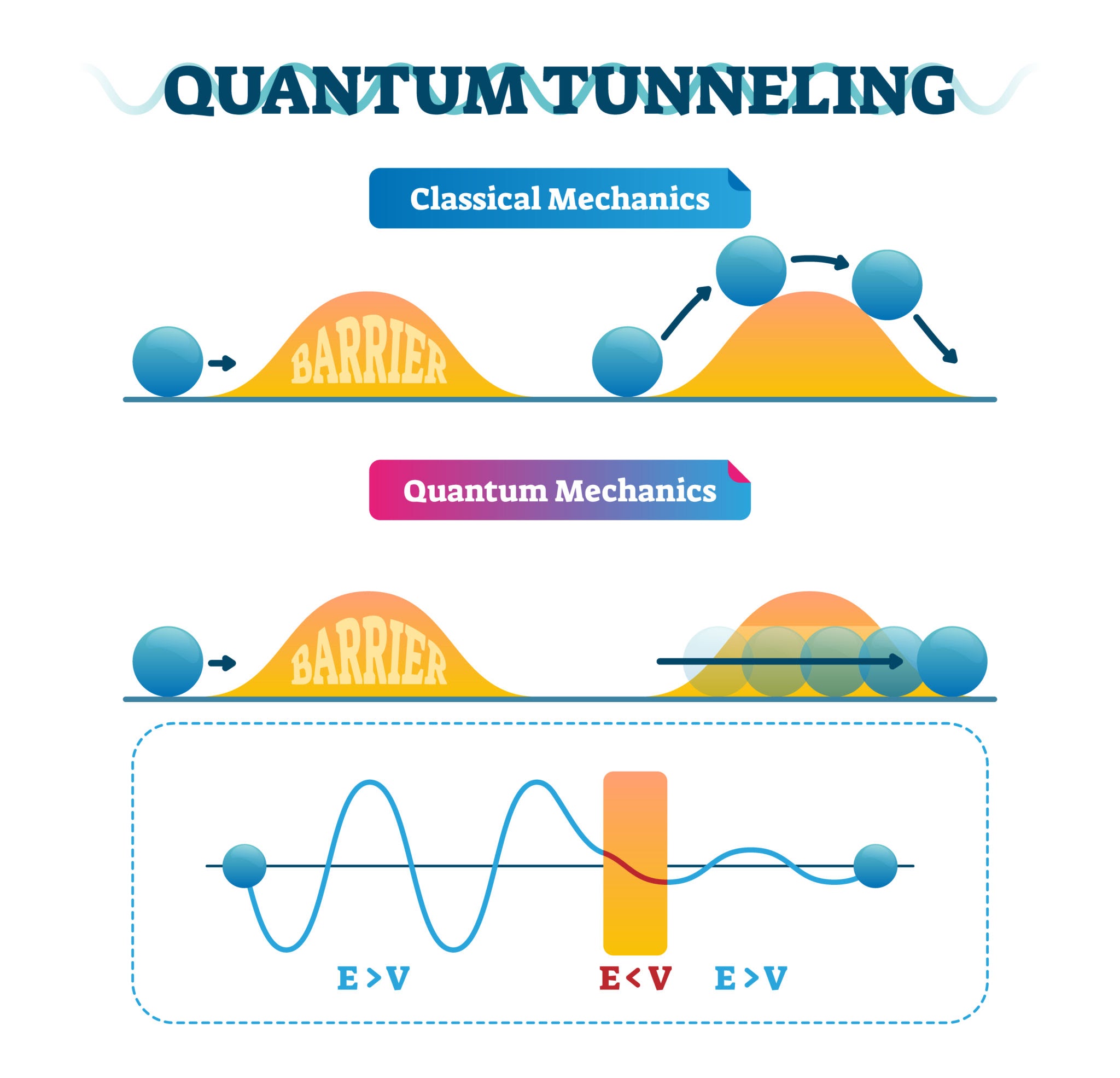
Fig 1: Classical particle is blocked (top), while Quantum wavefunction penetrates the barrier (bottom).
2. How It Works (The Mechanism)
The mathematical explanation lies in the solution to the Schrödinger equation inside the barrier region ($0 < x < a$).
The wave function in this region is given by:
$$ \psi(x) = C e^{-\kappa x} $$
Where the decay constant is $\kappa = \frac{\sqrt{2m(V_0 - E)}}{\hbar}$.
Key Concept: The wave function decays exponentially but does not reach zero immediately. This "leaking" of the wave function allows probability amplitude to exist on the other side of the barrier.
The probability of tunneling depends on:
- Width ($a$): A wider barrier causes more decay, reducing transmission.
- Mass ($m$): Heavier particles decay faster, making tunneling negligible for macroscopic objects.
3. Real-World Applications
- Alpha Decay: Radioactive particles tunnel out of the nucleus despite the strong nuclear force holding them in.
- Nuclear Fusion in Stars: Protons tunnel through the electrostatic repulsion barrier to fuse and release energy, powering the Sun.
- Scanning Tunneling Microscope (STM): Electrons tunnel across a vacuum gap between a sharp tip and a surface, allowing us to image individual atoms.
Question 1: The Rectangular Potential Barrier (tunneling)
Problem Statement: Consider a particle of mass $m$ and energy $E$ approaching a one-dimensional rectangular potential barrier of height $V_0$ and width $a$ (where $0 < x < a$). We consider the case where the particle's energy is less than the barrier height ($E < V_0$).
(a) Schrödinger Equations for the Three Regions
The potential $V(x)$ is defined as:
$$ V(x) = \begin{cases} 0 & \text{for } x < 0 \quad (\text{Region I}) \\ V_0 & \text{for } 0 < x < a \quad (\text{Region II}) \\ 0 & \text{for } x > a \quad (\text{Region III}) \end{cases} $$
Region I ($x < 0$) and Region III ($x > a$)
In these regions, $V(x) = 0$. The Time-Independent Schrödinger Equation is:
$$ \frac{d^2\psi}{dx^2} + \frac{2mE}{\hbar^2}\psi = 0 $$
Let $k^2 = \frac{2mE}{\hbar^2}$. The equation becomes:
$$ \frac{d^2\psi}{dx^2} + k^2\psi = 0 \quad \dots(1) $$
Region II ($0 < x < a$)
In this region, $V(x) = V_0$. Since $E < V_0$, the term $(E - V_0)$ is negative. We rewrite the equation as:
$$ \frac{d^2\psi}{dx^2} - \frac{2m(V_0 - E)}{\hbar^2}\psi = 0 $$
Let $\kappa^2 = \frac{2m(V_0 - E)}{\hbar^2}$ (where $\kappa$ is real). The equation is:
$$ \frac{d^2\psi}{dx^2} - \kappa^2\psi = 0 \quad \dots(2) $$
(b) Wave Functions and Boundary Conditions
General Solutions
- Region I ($x < 0$): The solution is oscillatory.
$$ \psi_1(x) = A e^{ikx} + B e^{-ikx} $$ (Incident wave + Reflected wave) - Region II ($0 < x < a$): The solution is exponential.
$$ \psi_2(x) = C e^{\kappa x} + D e^{-\kappa x} $$ - Region III ($x > a$): The solution is oscillatory.
$$ \psi_3(x) = F e^{ikx} + G e^{-ikx} $$ Since there is no reflection from $x = +\infty$, we set $G = 0$. Thus: $$ \psi_3(x) = F e^{ikx} $$
Applying Boundary Conditions
The wave function $\psi$ and its derivative $\frac{d\psi}{dx}$ must be continuous at boundaries $x=0$ and $x=a$.
At $x = 0$:
- Continuity of $\psi$: $ \psi_1(0) = \psi_2(0) \implies A + B = C + D \quad \dots(3) $
- Continuity of $\psi'$: $ \psi_1'(0) = \psi_2'(0) \implies ik(A - B) = \kappa(C - D) \quad \dots(4) $
At $x = a$:
- Continuity of $\psi$: $ \psi_2(a) = \psi_3(a) \implies C e^{\kappa a} + D e^{-\kappa a} = F e^{ika} \quad \dots(5) $
- Continuity of $\psi'$: $ \psi_2'(a) = \psi_3'(a) \implies \kappa(C e^{\kappa a} - D e^{-\kappa a}) = ik F e^{ika} \quad \dots(6) $
(c) Transmission Coefficient ($T$)
The Transmission Coefficient is $T = \frac{|F|^2}{|A|^2}$. We need to express $A$ in terms of $F$.
Step 1: Solve for C and D in terms of F
From equations (5) and (6), we can isolate $C$ and $D$:
$$ 2C e^{\kappa a} = \left( 1 + \frac{ik}{\kappa} \right) F e^{ika} \implies C = \frac{F}{2} \left( 1 + \frac{ik}{\kappa} \right) e^{ika} e^{-\kappa a} $$
$$ 2D e^{-\kappa a} = \left( 1 - \frac{ik}{\kappa} \right) F e^{ika} \implies D = \frac{F}{2} \left( 1 - \frac{ik}{\kappa} \right) e^{ika} e^{\kappa a} $$
Step 2: Substitute into Boundary Conditions at $x=0$
From equations (3) and (4), we can solve for $A$: $$ 2A = C\left(1 - i\frac{\kappa}{k}\right) + D\left(1 + i\frac{\kappa}{k}\right) $$
Substituting the values of $C$ and $D$ derived above:
$$ \frac{A}{F} e^{-ika} = \frac{1}{4} \left[ \left(1 + \frac{ik}{\kappa}\right)\left(1 - \frac{i\kappa}{k}\right) e^{-\kappa a} + \left(1 - \frac{ik}{\kappa}\right)\left(1 + \frac{i\kappa}{k}\right) e^{\kappa a} \right] $$
Simplifying the bracketed terms and grouping by Real and Imaginary parts using hyperbolic functions ($\cosh \kappa a$ and $\sinh \kappa a$):
$$ \frac{A}{F} e^{-ika} = \cosh(\kappa a) - i \frac{k^2 - \kappa^2}{2k\kappa} \sinh(\kappa a) $$
Step 3: Calculate the Modulus Squared
$$ \left| \frac{A}{F} \right|^2 = \cosh^2(\kappa a) + \left( \frac{k^2 - \kappa^2}{2k\kappa} \right)^2 \sinh^2(\kappa a) $$
Using $\cosh^2 x = 1 + \sinh^2 x$ and substituting $k^2 = \frac{2mE}{\hbar^2}$ and $\kappa^2 = \frac{2m(V_0 - E)}{\hbar^2}$, we get:
$$ \frac{1}{T} = 1 + \frac{V_0^2}{4E(V_0 - E)} \sinh^2(\kappa a) $$
Final Result: The Transmission Coefficient is given by: $$ T = \left[ 1 + \frac{V_0^2}{4E(V_0 - E)} \sinh^2(\kappa a) \right]^{-1} $$
Discussion: Quantum Tunneling
- Effect of Width ($a$): Since $\sinh^2(\kappa a)$ grows exponentially with $a$, the transmission $T$ decreases exponentially as the barrier width increases.
- Effect of Mass ($m$): Since $\kappa \propto \sqrt{m}$, heavier particles result in a larger $\kappa$, making $T$ vanish rapidly. This explains why tunneling is significant for electrons but not for macroscopic objects.
Time Remaining: 900s